Dr. Chang Liu was my advisor and principal investigator at the FLUids, rEduction, Nonlinearity, and Turbulence (FLUENT) Lab for two and half years of my undergraduate career.

You might be wondering why a roboticist did a thesis related to fluid dynamics. And the answer is, they actually have a lot more in common than meets the eye. I found my project super interesting because it combined two of my interests, control theory and environmental science.

The goal of my research was to study techniques for stability analysis of time-dependent dynamical systems. I applied numerical Lyapunov analysis to study the stability of shear flows in the Arctic Ocean. Understanding the dynamics of these shear flows has important implications for climate science and sea ice melt.

I implemented several stability analysis methods to compare their efficacy (Lyapunov, ode45, Floquet theory). I ran countless simulations on high performance computing clusters using MATLAB and SLURM.

At the conclusion of my undergraduate degree, Dr. Liu and I published a paper based on my thesis in the 2026 American Control Conference (ACC).

Want to learn more?

Here are a few modified exerpts, with some commentary, from my thesis if you want to get a better understanding of the applications. I tried to make it as easy to understand as possible.

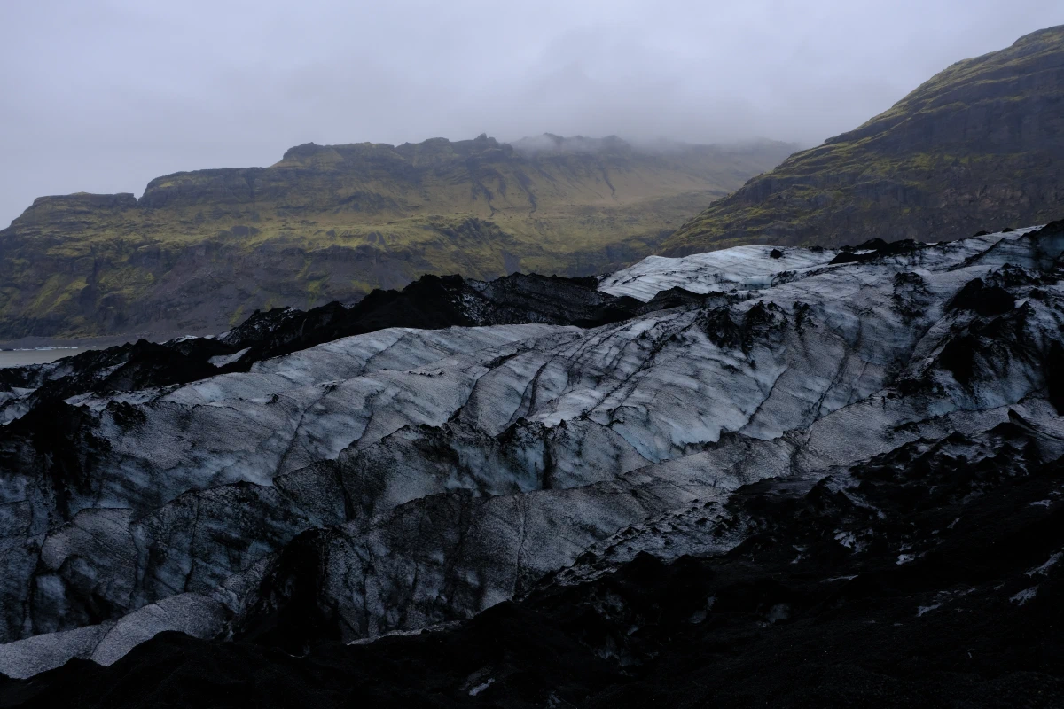
The de-oxygenation of the ocean through warming and freshening of waters, as well as increased acidity due to the absorption of CO2, are stressing marine ecosystems across the globe [2]. Recent literature shows that almost all five of Earth’s global mass extinction events have evidence of global warming, ocean acidification, and de-oxygenation occurring from impaired carbon cycle function [3]. […] The mechanisms in the ocean dynamics that limited sea ice melt are diminishing at an alarming rate [4] causing rapid sea ice melt, sea level rise, and influx of fresh water.

Warming waters = melting glaciers = fresher waters and sea level rise = deoxygenation which is harmful for marine life.

These trends are a result of global ocean mixing processes known as Thermohaline Circulation. Atlantic Ocean currents that are warm and salty are transported to the Arctic Ocean at a depth of 150-900 meters [5]. This transported water mass releases heat to the surface causing sea ice melt. Today, this accumulation of thermal mass [in the Arctic Ocean] contains more than enough heat to melt all sea ice in the Arctic Ocean several times over [5]

Obviously we still have glaciers (for now). So the question scientists want to answer is why hasn’t the heat below the surface radiated upwards yet?

The root cause of the phenomenon that has slowed heat transport up to now, known as thermohaline staircasing, still has not been understood for more than fifty years [4]

Unfortunately this is not a settled debate. But our technique may offer advantages compared to existing techniques.

Unlike numerical simulation, Lyapunov-based stability analysis does not require extensive simulations, but directly characterizes the solution trajectory for a set of initial conditions. It can also be applied to a wide class of systems that other “simulation-free” methods can’t handle.

So what does stability mean and why is it relevant to thermohaline staircasing?

Lets first start with what stability means. You can think of it as objects ability to restore itself to an initial state/equilibrium.

For example, imagine a ball initially at the crest of a hill. The ball is at an equilibrium because it isn’t moving anywhere. But with a small nudge, suddenly the ball releases all of its potential energy into kinetic energy. This is known as an unstable equilibrium. It doesn’t take much to perturb the ball into a new state.

Now consider the same ball, but it’s located at the valley of an infinitely tall hill. You can kick the ball as hard as you can but the ball will always eventually roll back down to the bottom of the hill. This is known as a stable equilibrium (technically speaking it is globally asymptotically stable equilibrium… there are lots of fancy names for this stuff).

I hope that makes sense. So now lets consider another thought experiment to see why thermohaline staircasing is so weird. It’s a bit of an oversimplification just for the record.

Lets say you go to the bar and get one of those tasty mixed drinks with lots of layers. This is akin to the thermohaline staircasing in the Arctic Ocean, except the layers have different temperature/salinity content. Now if you shook your mixed drink, the drink would become much less interesting. It doesn’t take much shaking to make the uniformally mixed. This layered state is considered an unstable equilibrium. With a small nudge, the layers likely disappear.

Now this is where things get freaky. Imagine you start with a uniformally mixed drink and shake it around a whole bunch. You would expect that the drink would look virtually identical to how it started. Of course it would… what am I? Crazy? The mixed state is the stable equilibrium.

But what if the drink didn’t look the same. In fact, your shaking actually caused layers to spontaneously form. Order spontaneously appears from disorder. It feels impossible, at least to me. But this is what happens in specific ocean conditions. Somehow this “unstable” equilibrium forms and it sticks around. The scary part is that this “unstable” equilibrium is the only thing between us and every glacier in the Arctic Ocean being melted.

One theory as to why the layers form is because of the periodic nature of the tide. Water isn’t perfectly still. So maybe somehow the tide going in and out makes this layered state persist. This time-dependent scenario is what I studied. And it is much harder to figure out stability if the dynamics of the system are constantly changing. This is common in fluid dynamics.

So how do you figure out stability?

In many cases people “cheat” and simulate the physics on supercomputers to determine if the system is stable. I say cheat because simulating the physics doesn’t actually guarantee the system is actually stable. The computer would have to try an infinite number of starting conditions in its simulation in order to get a definite answer. Practically speaking, the numerical simulation is often enough.

But Lyapunov stability analysis is a very interesting tool because it does not require simulating every possible scenario. Somehow you can extract whether a system is stable for all conditions without simulating a single particle of the system. It feels like a bit like magic.

The amazing part is that you already know how it works. At least using the analogy with the ball on the hill I told you about. You can identify if the dynamics of the system, more specifically the energy, are valley-like or crest-like. Again, I’m oversimplifying some things but it gets the idea across.

In other words, is it a rightside up parabola $x^2$ or an upside down parabola $-x^2$.

In this case it isn’t a one-dimensional parabola. It’s a multi-dimensional paraboloid, and I can use linear algebra to express it. For instance

$$ \begin{gather*} p_1 x_1^2 + p_2 x_2^2 + \dots + p_n x_n ^2 = 0 \\ \vec{x}^T \mathbf{P} \vec{x} = 0 \\ \end{gather*} $$

And $\mathbf{P}$ is

$$ \mathbf{P} = \begin{bmatrix} a_1 & 0 & 0 & \cdots & 0 \\ 0 & a_2 & 0 & \cdots & 0 \\ 0 & 0 & a_3 & \cdots & 0 \\ \vdots & \vdots & \vdots & \ddots & \vdots \\ 0 & 0 & 0 & \cdots & a_n \end{bmatrix} $$

Do the matrix multiplication out. You’ll see that the expressions are equivalent. This is known as a quadratic form. And fun fact, if you wanted to have cross terms, like $x_1 x_3$, you can put entries in the off diagonal entries of the matrix to achieve this.

Derivation for time-independent system

Let me sketch out how the Lyapunov method works. This is for a time-independent system. Using Lyapunov analysis for this setup is overkill and much more difficult than doing an eigenvalue analysis (stable if all eigenvalues have negative real components). But extending this to a time-dependent system has similar flavors.

Lets say we have a differential equation $\frac{d \vec{x}}{dt}= \mathbf{A}\vec{x}$. You can write the energy of the linear system as a quadratic form $V=x^{T}\mathbf{P}x$. If a system is stable, then the energy will decay to an equilibrium.

$$ \begin{align*} \frac{dV}{dt} < 0 \\ \dot{x}^{T}\mathbf{P}x + x^{T}\mathbf{P}\dot{x} < 0 \\ \end{align*} $$

We know that $\dot{x}=\textbf{A}x$ so

$$ \begin{align*} (\textbf{A}x)^{T}\mathbf{P}x + x^{T}\mathbf{P}(\textbf{A}x) < 0 \\ x^{T}(\mathbf{A}^{T}\mathbf{P} + \mathbf{P}\mathbf{A})x < 0 \end{align*} $$

In order for this inequality to hold true, $\mathbf{A}^{T}\mathbf{P} + \mathbf{P}\mathbf{A}$ is negative definite, which is like the upside down parabola.

So if we can find $\mathbf{P}$ (assuming it is positive semidefinite) so that the inequality holds true: $$ \mathbf{A}^{T}\mathbf{P} + \mathbf{P}\mathbf{A} \prec 0 $$

Then we know the system is stable.

I am going to pull a few expressions out of a hat. If you want to see the full derivation I suggest reading the ACC paper.

If the system is unstable, then it is bounded by an exponential. The trajectory is bounded by an exponential when

$$ \mid\mid x(t)\mid\mid \leq e^{c\lambda t}\mid\mid x(0)\mid\mid $$

This comes from the differential equation $\frac{dV}{dt}<2\lambda V$ which has an exponential solution. $$ \begin{align*} \frac{dV}{dt}-2\lambda V < 0 \\ x^{T}(\mathbf{A}^{T}\mathbf{P} + \mathbf{P}\mathbf{A})x -x^{T}2\lambda \mathbf{P}x <0 \\ x^{T}(\mathbf{A}^{T}\mathbf{P} + \mathbf{P}\mathbf{A} - 2\lambda \mathbf{P})x <0 \\ \\ \mathbf{A}^{T}\mathbf{P} + \mathbf{P}\mathbf{A} < 2\lambda \mathbf{P} \end{align*} $$ Therefore we can also find the growth rate of the instability if we find a matrix $\mathbf{P}$ that satisfies the inequality involving lambda.

It is pretty challenging to find $\mathbf{P}$. There isn’t an algorithmic way to find an analytical solution. So it’s a lot of guess and check. But if we use convex optimization, we can find $\mathbf{P}$ numerically. And same goes for the time-dependent system.

Conclusion

Please feel free to email me if you have any questions. And if you’d like me to explain my work in more detail in another post I’d be happy to share.